0. Quickstart — from raw data to a figure in five steps
New to SpectraFit XPS? This is the whole workflow in miniature. Brackets link to the detailed section.
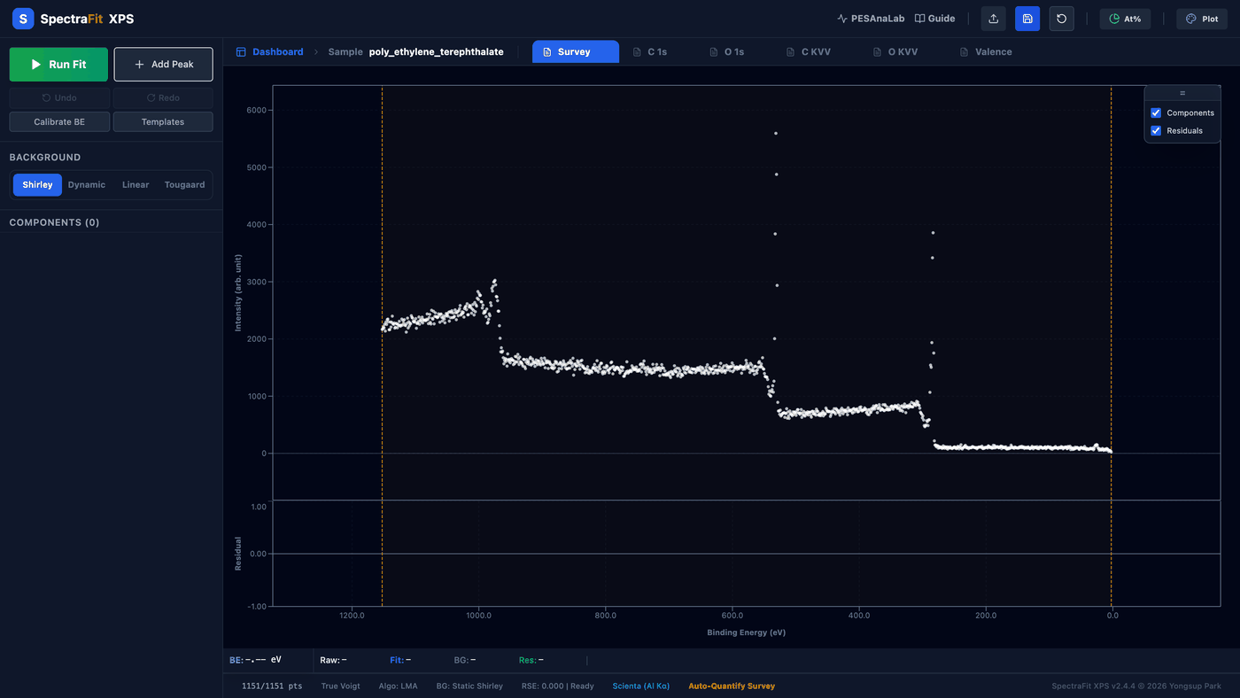
Figure 1 — The SpectraFit XPS workspace. Full application window with poly(ethylene terephthalate) (PET) loaded and the Survey tab active. Shows the region tab bar (Survey · C 1s · O 1s · C KVV · O KVV · Valence), the left sidebar (Run Fit / Add Peak, the BACKGROUND selector, and the COMPONENTS list), the central spectrum panel with the gold ROI handles, the lower residual panel, and the footer status bar (point count, line-shape, background type, RSE, and the auto-detected instrument = Scienta).

The header toolbar. Left to right: PESAnaLab and Guide links, Open / Import, Save / Export, Reset, the At% quantification panel, and the Plot (Publication Plotter) toggle.
- Load your data. Drag a file onto the window, or use Open. VAMAS (
.vms), Excel, CSV/Text, and several vendor formats are supported. Multi-region and depth-profile files open as separate tabs/slices automatically. [→ §2] - Set the region of interest (ROI). Drag the two gold handles to bracket your peak(s). Everything outside the shaded band is excluded from the fit. [→ §3]
- Choose a background. Pick Shirley (default for most core levels), Linear, Dynamic Shirley, or Tougaard. [→ §3.2]
- Add and position peaks. Add a peak, then drag its apex handle — horizontal = binding energy, vertical = height. Arrow keys give fine steps. Add spin–orbit partners with the Doublet icon. [→ §4]
- Fit and export. Click Run Fit. When the residual looks flat, open the Publication Plotter and export SVG for journals or PNG for slides. [→ §5, §7, §9]
Tip: a good fit shows a flat, structureless residual in the lower panel. Structured wiggles mean a missing or mis-shaped component.
1. Introduction: the SpectraFit XPS philosophy
Traditional XPS software often suffers from steep learning curves or outdated interfaces. SpectraFit XPS is built around three principles of interactive precision:
- Real-time feedback: as you drag peaks or adjust ranges, the background and residuals update instantly.
- Mathematical integrity: while many tools rely on pseudo-Voigt approximations, SpectraFit XPS uses high-fidelity line-shape calculations, including the Doniach–Sunjic (DS) profile for asymmetric metallic lines.
- Workflow efficiency: from mosaic dashboard overviews to granular publication styling, the app takes you from raw data to a finished figure in minutes.
2. Data management & persistence
2.1 Multi-format import
SpectraFit XPS handles a wide range of scientific data formats:
- VAMAS (.vms): full support for ISO 14976 files, including automatic region splitting and transmission-function correction at load time.
- Excel (.xlsx / .xls): structured spreadsheets with Binding Energy and Count columns.
- Text / CSV: standard tab-separated or comma-separated files.
- XPS ASCII (.asc): two-column files delimited by semicolon, comma, or
whitespace; lines beginning with
#are treated as comments. - MRS (.mrs): Physical Electronics format with key=value metadata; sample description, scan count, operator, and timestamp are extracted automatically.
- VG-Microtech (.1): fixed-format text files with an 8-parameter header line; pass energy and photon energy are extracted automatically.
- Parameter files (.par / .json): these do not contain spectral data; instead they store the entire fitting model — peak positions, widths, constraints, and background settings.
- Project files (.sfitx): introduced in Ver. 1.80, these capture the complete state of a session — single spectrum, multi-region spectra, multi-region depth-profile data, and multiple samples. Reopening restores the entire session. The format is JSON, conventionally named "Project_Name.sfitx".
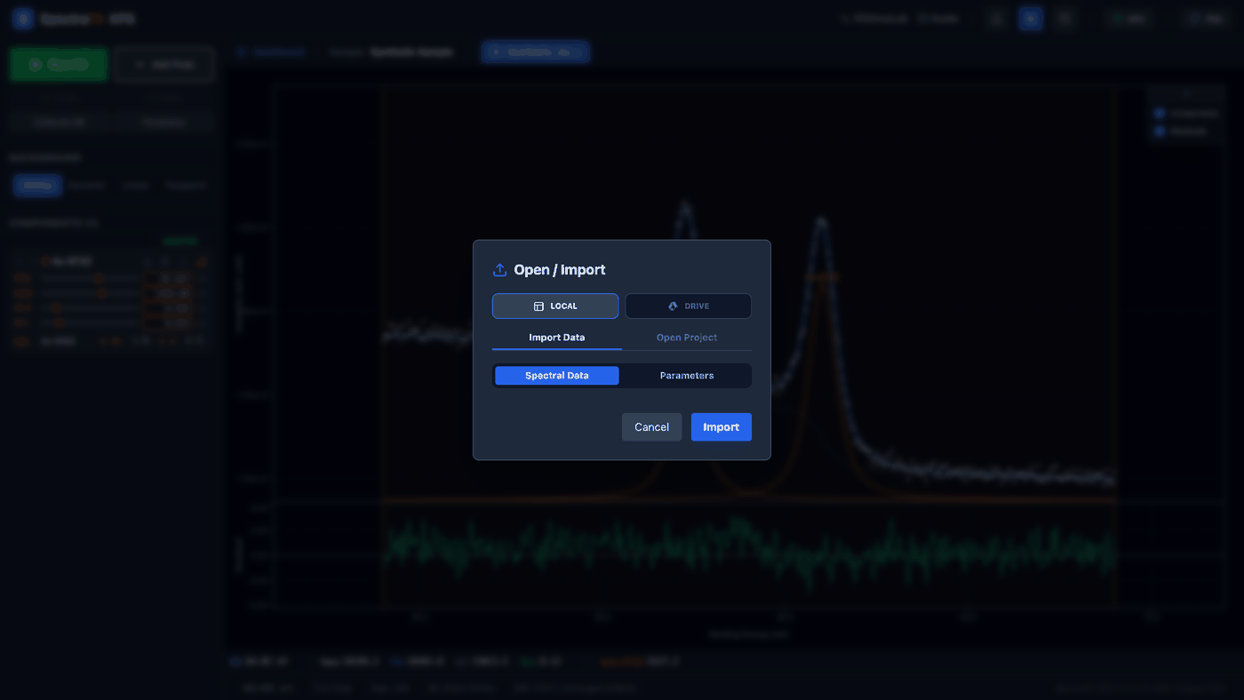
The Open / Import dialog (the upload icon in the header). Choose
Local or Google Drive as the source, then Import Data (spectral
files or .par parameter sets) or Open Project (.sfitx).
2.2 Modern file-system integration
Starting with v1.71, SpectraFit XPS uses the Web File System Access API:
- Choose your folder: saving and opening invoke the standard OS "Save As" / "Open" dialogs — you are no longer restricted to the browser's Downloads folder.
- Location memory: the app assigns a unique session ID (
spectra-fit-picker) to its file dialogs, so the browser remembers the last folder used.
3. Region of Interest (ROI) selection
Defining the ROI is the first step in any fit.
3.1 Selection mechanics
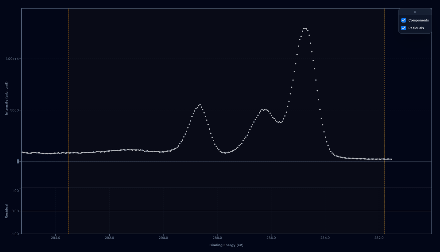
Figure 2 — ROI selection on the PET C 1s region. The C 1s region with the two vertical gold ROI handles set by double-clicking at ≈ 293.5 eV and ≈ 281.8 eV, bracketing the C 1s envelope. Raw data only (dots) — no components yet — so only the spectrum and the region of interest are shown; everything outside the gold band is excluded from the fit.
- Visual selection: drag the gold handles at the edges of the spectrum, or double-click to move the nearest ROI edge to the clicked point.
- Excluded data: points outside the gold region are ignored by the LMA optimizer, ensuring noise or adjacent peaks do not bias the result.
3.2 Advanced background modeling
The background represents the inelastic-scattering contribution to the signal. Select a model from the background bar; the choice updates the fit in real time:

Figure 3 — Background-model selector. A close crop of the BACKGROUND control showing the four options — Shirley (highlighted), Dynamic, Linear, Tougaard.
- Shirley — the industry standard for metallic and semi-metallic regions.
- Linear — a straight baseline between the ROI endpoints. Best for flat, well-isolated peaks or quick previews where a full Shirley/Tougaard model is unnecessary.
- Dynamic Shirley — the background slope and intercept become active parameters in the LMA fit, so the background evolves alongside the peaks. Rare and powerful.
- Tougaard — a physics-based model accounting for the energy-loss cross-section; preferred for wide-range scans. When selected, parameter fields appear in the sidebar. It supports both the 2-parameter form (B, C) and the 4-parameter U4 form (B, C, C′, D), with a one-click Universal Preset (B = 2866, C = 1643, C′ = 1, D = 1).
- Smart cleanup — when all peaks are removed, the background line disappears automatically, keeping the workspace tidy.
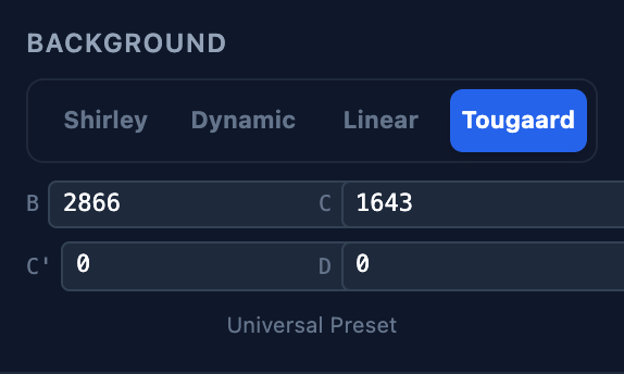
Tougaard parameters. Selecting Tougaard reveals the B, C, C′, D fields and the one-click Universal Preset directly beneath the selector.
4. Peak fitting & constraints
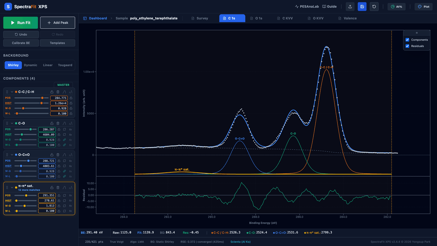
Figure 4 — PET C 1s resolved into four chemical-state components. The headline fitting figure. White dots = raw data; blue line = sum-fit envelope; grey dashed = Shirley background; and four True-Voigt components —
- ≈ 284.8 eV — C–C / C–H (aromatic ring + backbone carbons); the tallest peak, the Master, and the intensity reference.
- ≈ 286.3 eV — C–O (ester single-bonded carbon, –O–CH₂–).
- ≈ 288.7 eV — O–C=O (ester carbonyl carbon).
- ≈ 291.4 eV — π→π* shake-up satellite (broad and weak; its widths were unlinked from the master so it can broaden independently).
Nominal area ratio C–C/H : C–O : O–C=O ≈ 3 : 1 : 1; the shake-up a few %. The slave FWHMs stay linked to the master (one shared width) and the residual panel is close to structureless (RSE ≈ 0.37). Binding energies are as-measured on this Scienta dataset — use Calibrate BE (§4.4) to place C–C/C–H exactly on the 284.8 eV charge reference if desired.
4.1 Peak architectures
- True Voigt: a rigorous convolution of Gaussian (instrumental and thermal broadening) and Lorentzian (lifetime broadening) profiles.
- Doniach–Sunjic (DS): for metallic peaks where electron–hole-pair excitation produces a characteristic tail on the high-binding-energy side.
- SGL (Sum Gaussian–Lorentzian): added for CasaXPS compatibility; a dedicated MIX slider (0–100 %) controls the Gaussian–Lorentzian ratio. The MIX value is held fixed during fitting (only position, height, and FWHM are optimized), matching CasaXPS behavior.
- Doublets (spin–orbit splitting): click the Doublet icon to add a partner peak. SpectraFit looks up the orbital type (p, d, f) and applies standard physical rules (e.g., 2:1 area ratio for p-orbitals, characteristic energy separations). The SO splitting and intensity ratio can each be locked or unlocked individually; when unlocked, they become free fitting parameters.
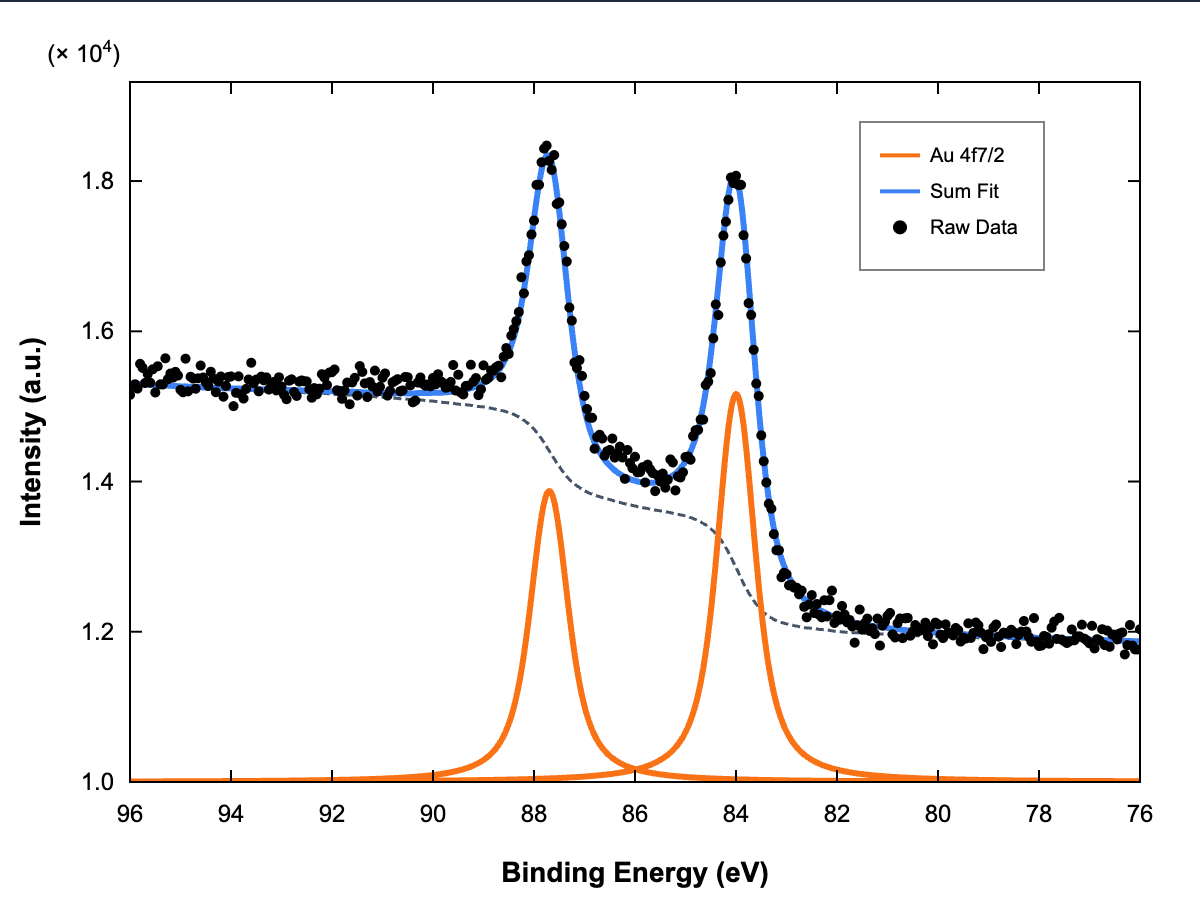
Figure 5 — Spin–orbit doublet: synthetic Au 4f. A clean illustration of spin–orbit splitting using the app's built-in synthetic Au 4f sample (it loads automatically when the app opens with no file). Two orange components — Au 4f₇/₂ at ≈ 84.0 eV and Au 4f₅/₂ at ≈ 87.7 eV — separated by the characteristic ≈ 3.7 eV spin–orbit splitting and held at the 4 : 3 area ratio (4f₇/₂ : 4f₅/₂) by the doublet rule. Blue = sum fit, grey dashed = Shirley background, black dots = raw data; rendered white-background in the Publication Plotter. On any real p/d/f peak, clicking the Doublet icon generates the partner automatically.
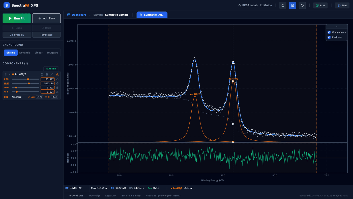
The doublet in the workspace. The same synthetic Au 4f after Run Fit: the master card carries a dashed DBL row with the partner name, the ΔE spin–orbit separation, and the R intensity ratio — each with its own lock/unlock toggle (see also §4.1 "Doublets").
4.2 The Master Peak concept
The first peak in your list serves as the Master:
- Linking: click the Link (chain) icon on any slave peak to tie its width, position delta, or height ratio to the Master.
- Global adjustment: when a parameter is linked, dragging the Master moves all linked components in synchrony, preserving the physical relationships of your chemical model.
- Expression-based constraints (Ver 2.1): any secondary peak can reference
another through an expression — for example
P1.pos + 1.18orP1.fwhm_g * 1.2. Supported for position, height, fwhm_g, fwhm_l, and asymmetry, and re-evaluated at every fitting iteration.
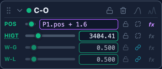
Expression constraints. Clicking the fx toggle on a slave-peak
parameter opens the purple expression field — here the C–O position is tied
to the master with P1.pos + 1.6. The cyan chain icons on W-G / W-L show
those widths are linked to the Master.
4.3 Interactive handles
You do not need to type numbers to find a good starting point.
- Circular handles: every peak carries a handle at its apex. Drag horizontally to change the binding energy (position) and vertically to change the intensity (height).
- Arrow keys: select a peak and use the keyboard arrows for fine increments.
- Drag-and-move editing (Ver 1.72): clicking and dragging a component peak is equivalent to grab-and-move with the arrow keys.
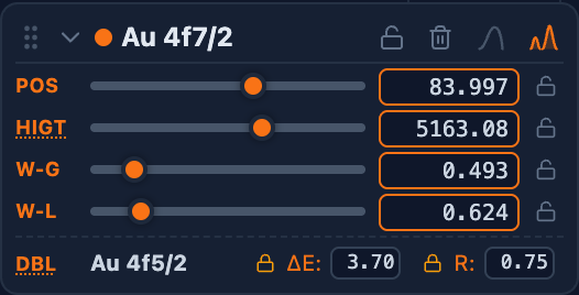
The component card. POS / HIGT / W-G / W-L sliders with numeric fields and per-parameter lock toggles; top-right are the whole-peak lock, delete, line-shape cycle (Voigt → DS → SGL), and Doublet buttons. Clicking HIGT toggles an AREA readout, and the dashed DBL row appears when a doublet is active.
4.4 BE calibration & peak-model templates
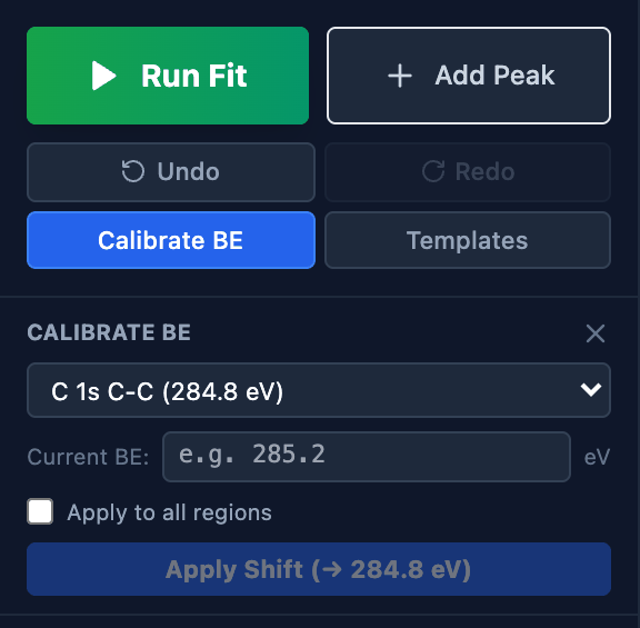
Calibrate BE (sidebar) applies a rigid binding-energy shift: pick a reference (C 1s 284.8 · C 1s NIST 284.6 · Au 4f₇/₂ · Ag 3d₅/₂ · Cu 2p₃/₂), type the position you actually measured, and Apply Shift — optionally to all regions of the sample at once.
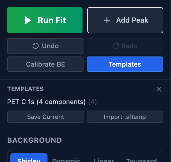
Templates saves the current multi-peak model for reuse (stored in the
browser; export/import as .sftemp JSON) — here the four-component
"PET C 1s" model from Figure 4, ready to load onto the next PET sample.
5. The optimization engine
5.1 Levenberg–Marquardt optimization
Click Run Fit to begin the iterative optimization. The engine computes the Jacobian of your model and steps through parameter space to minimize the Residual Standard Error (RSE).
- Early convergence: the loop monitors iteration-to-iteration improvement; if a cycle improves the fit by less than 10⁻⁶, the process terminates early, keeping the experience snappy even with complex models.
- Fast Math mode (Ctrl + F): toggles optimized mathematical approximations that significantly accelerate the fit, particularly useful for multi-peak DS models.
5.2 Residual analysis
The residual plot at the bottom is the primary tool for validating a fit.
- Linear connection — only real data points are shown, joined by linear segments. This avoids the "smoothed-curve illusion" and faithfully reflects the instrument noise floor.
- RSE monitoring — the footer status bar reports the quantitative fit error. A flat residual with no structured features indicates a mathematically sound model.


The status rows. Hovering the chart fills the live readout (BE, raw counts, fit, background, residual, and each component's value at the cursor); the footer reports the ROI point count, line-shape, algorithm, background type, RSE, fit convergence, and the auto-detected instrument.
6. Navigation & zooming
6.1 Mouse-anchored zoom
- Anchor point: scrolling the mouse wheel while hovering over the chart expands and contracts the view relative to the data point under the cursor, letting you zoom directly into a small feature.
- Reset Zoom button: a Reset Zoom button in the upper-left corner of the plot restores the default Y-zoom in one click.
6.2 Depth-profile slider
For samples with multiple etch levels, the Depth-Profile Slider at the top of the main area lets you navigate slices instantly. Use the ← / → arrow keys for rapid frame-by-frame comparison.
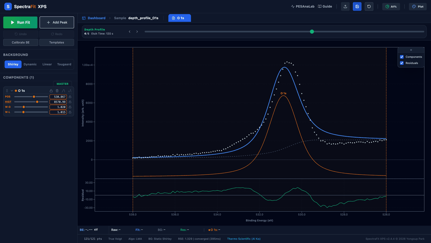
Depth-profile navigation. A multi-block VAMAS file (the same region
measured at successive etch levels) opens with the emerald Depth Profile
strip — here slice 4/6 of a synthetic O 1s profile, with its etch-time label,
arrow steppers, and slider. (Demo file: sample_data/depth_profile_O1s.vms,
regenerable with node scripts/gen_depth_profile_vms.mjs.)
6.3 The sample dashboard
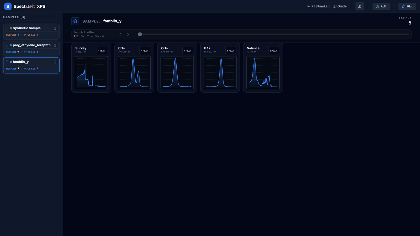
Dashboard view. The Dashboard breadcrumb lists every loaded sample on the left with its region and profile counts; the mosaic shows one mini-chart per region of the selected sample. Click any card to jump straight to that region's fitting view.
7. The Publication Plotter
The Publication Plotter is a dedicated design environment that turns your analysis into a figure ready for a high-impact journal.
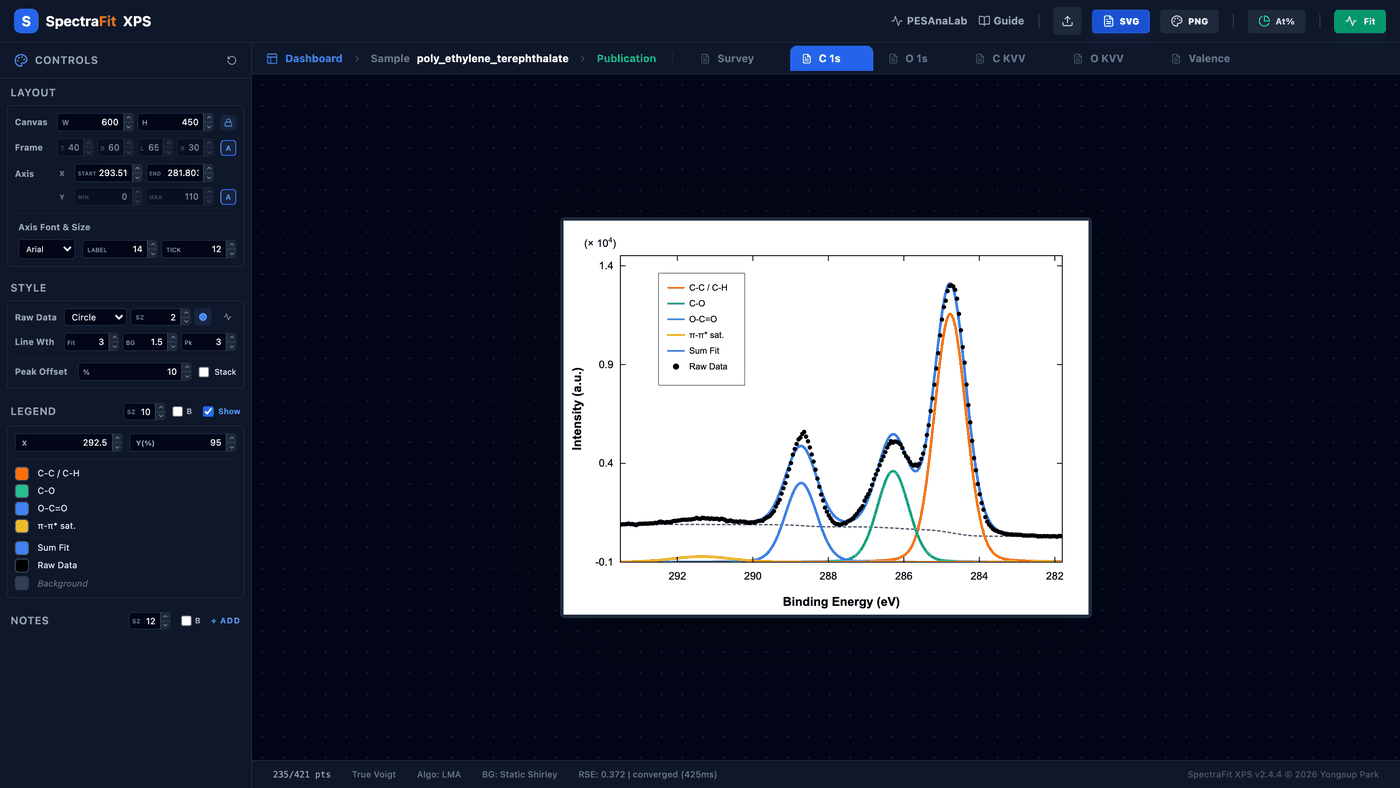
Figure 6 — The Publication Plotter. The Figure-4 fit rendered on a white canvas, with the design sidebar: canvas size and frame margins, axis ranges and fonts, raw-data symbol and line widths, the positionable legend, and text annotations. In this view the header actions become SVG and PNG export buttons.
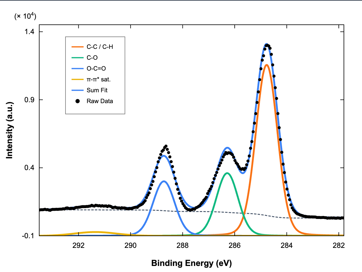
The finished figure. Black filled circles = raw data, blue = sum fit, coloured lines = the four components, a reversed "Binding Energy (eV)" x-axis (high → low), an "Intensity (a.u.)" y-axis, and the legend moved clear of the peaks — the clean, light figure for slides and papers, replacing the dark in-app view.
7.1 Precision layout
- Dimension steps: the Width and Height spinners use a 0.5 % step.
- Aspect-ratio lock: enabled by default to ensure peaks are not accidentally stretched or squashed when the canvas is resized.
- Sync Auto-Y: the Auto-Y (A) button synchronizes the calculated automatic bounds back into the manual input fields, so auto-scale becomes a starting point for further manual refinement.
7.2 Styling & annotations
- Symbols: choose between "None" (lines only) and various markers — circles, squares, crosses — for raw data.
- Legends: drag and drop the legend coordinates; labels are fully customizable per component.
- Annotations: place text labels directly on the plot to highlight specific chemical states (Fe²⁺, SiO₂, …).
8. Quantification
Quantification was introduced in v1.90-beta and substantially expanded in v2.0 by integrating components of KherveFitting (BSD-3-Clause, by Gwilherm Kerherve, Imperial College London).
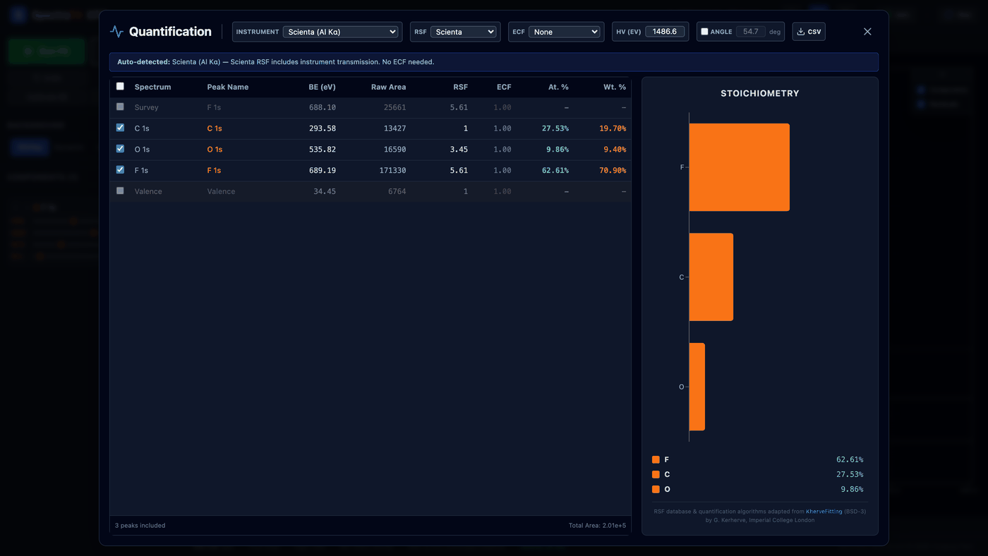
Figure 7 — Quantification of Fomblin Y (C, O, F). The Quantification
panel over the fitted fomblin_y.vms regions, with Peak Name, BE, raw Area,
RSF, ECF, At %, and Wt % beside the stoichiometry bar chart. The Scienta
preset was auto-detected from the VAMAS header (blue banner), so RSF and ECF
needed no manual setup. The fluorine-shifted C 1s (≈ 293.6 eV) is still
correctly named "C 1s" from its VAMAS region label. With the Survey and
Valence rows unchecked (they are not core-level regions), the three
core-level rows give C 27.5 / O 9.9 / F 62.6 at % — the
fluorine-dominated stoichiometry expected for this perfluoropolyether —
and fluorine dominates the Wt % column even more strongly.
Note — automatic identification scope. Automatic peak labelling and survey auto-quantification identify only commonly-encountered elements, via their core photoelectron lines, and they trust an explicit VAMAS region label (so a fluorine-shifted C 1s is still named "C 1s", and a valence-band region is named "Valence" rather than a spurious element). For samples containing rarer elements, set the peak name by hand from the peak-name dropdown, which searches the full database. As always, confirm the Peak Name column before trusting At %.
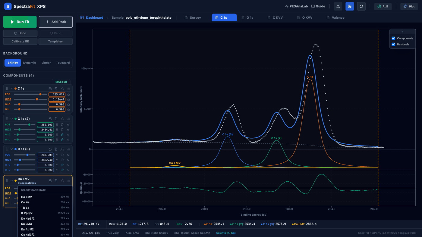
Correcting an auto-label. Here the PET π→π* shake-up at ≈ 291.4 eV was auto-labelled "Ca LM2" (an Auger-line coincidence). Selecting the peak and clicking N more matches under its name opens the candidate list — each with its database binding energy — for a one-click correction; or simply type any name by hand.
8.1 Quantification engine
- RSF database: instrument-specific Relative Sensitivity Factor sets adapted from KherveFitting, covering Thermo, Kratos, PHI, Scienta, Shimadzu, and more.
- TPP-2M IMFP calculator: Inelastic Mean Free Path computed from the Tanuma–Powell–Penn formula with average matrix parameters from Briggs & Grant.
- Energy Correction Factor (ECF) methods: five options — Scofield (KE^0.6), Wagner (KE^1.0), TPP-2M IMFP, EAL (Seah universal equation), and None.
- Angular correction: an L(β, θ) factor for non-magic-angle geometries, with an enable/disable checkbox and angle input (default 54.7°, the magic angle).
- Weight percent: atomic percentages are converted to weight percentages using standard atomic masses (H–U); a Wt % column is shown in the table.
8.2 Instrument auto-detection
- Automatic configuration: when a VAMAS file is loaded, the manufacturer is detected from the header and the Quantification Panel auto-configures the matching RSF, ECF, and photon energy.
- Manual preset selector: a dropdown of nine instrument presets is available when auto-detection cannot determine the source.
- Compatibility warnings: a blue banner confirms an auto-detected instrument; an amber banner warns of incompatible RSF/ECF combinations (e.g., a manufacturer-specific RSF combined with an ECF that would double-correct for transmission).

Compatibility warning. Combining the Scienta RSF set (which already includes the instrument transmission) with a TPP-2M ECF would double-correct — the amber banner names the conflict and the fix.
8.3 Survey auto-quantification
Wide-scan (survey) spectra are detected automatically when the BE range exceeds 500 eV. Clicking "Auto-Quantify Survey" in the status bar runs peak detection, element identification against the XPS database, and a quick At % calculation — all without performing a peak fit.
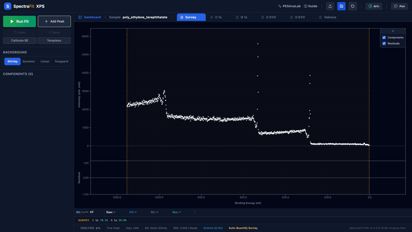
Survey auto-quantification. One click on Auto-Quantify Survey (amber, in the footer) reports C 1s 70.1 % / O 1s 29.9 % for the PET survey — matching the C₁₀H₈O₄ repeat unit (nominal 71 : 29 for C and O). See the v2.4.4 release notes for current reliability limits on complex multi-element samples.
9. Exporting & reporting
9.1 Graphic formats
- SVG (Scalable Vector Graphics): the preferred format for publications. SVGs scale infinitely in Adobe Illustrator or Inkscape without quality loss.
- PNG: high-resolution raster export for presentations and reports.
9.2 Data export
- The .fit file: a comprehensive text export containing binding energy, raw data, sum fit, background, and every individual component curve.
- Excel export: a structured .xlsx file that includes quantification results and area percentages.
- VAMAS export (.vms): added in Ver 2.3; spectrum data can be exported as ISO 14976 VAMAS files compatible with CasaXPS, KherveFitting, MultiPak, UniFit, and any other ISO-14976 reader.
- Project files (.sfitx): save and reload an entire fitting session in a single JSON file.
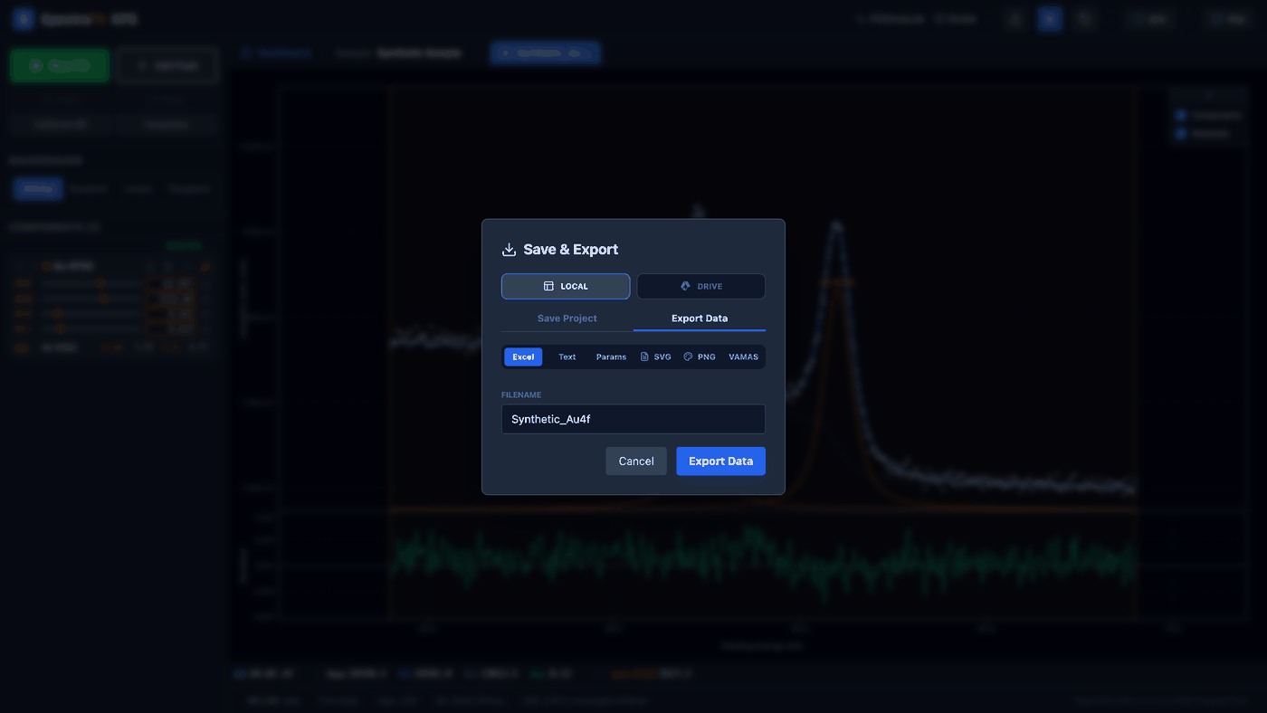
Save & Export (the blue save icon in the header). Save Project writes
the full .sfitx workspace; Export Data offers Excel, Text (.fit),
Params (.par), SVG, PNG, and VAMAS — saved to local disk or Google Drive.
10. Quick reference
| Action | Shortcut / gesture |
|---|---|
| Set / adjust ROI | Drag the gold handles, or double-click to move the nearest ROI edge |
| Reset view | Double-click the chart (resets Y-zoom and snaps the nearest ROI edge to the cursor) |
| Zoom in / out | Mouse wheel (anchored to the pointer) |
| Reset Y-zoom only | Reset Zoom button, upper-left of the plot |
| Add a peak | Click in the spectrum / use the add-peak control |
| Move a peak | Drag its apex handle (horizontal = position, vertical = height) |
| Fine-tune a peak | Select it, then use the arrow keys |
| Link a peak to the Master | Click the Link (chain) icon on the slave peak |
| Add spin–orbit partner | Click the Doublet icon |
| Run the fit | Run Fit button |
| Accelerate the fit | Ctrl + F (Fast Math toggle) |
| Undo / Redo | Ctrl + Z / Ctrl + Shift + Z (50-step history) |
| Navigate depth-profile slices | ← / → arrow keys (or the slice slider) |
| Calibrate binding energy | Calibrate BE button in the sidebar |
The first peak in the list is always the Master; linked slaves move with it.
11. Troubleshooting & FAQ
Google Drive shows an "unverified app" warning when I connect. Expected — Google verification can take weeks to months for small projects. The app only accesses files you explicitly open or save, and your data stays in your browser. If you'd rather not grant access, use local files; everything works identically.
My quantification doesn't match my instrument's software. Quantification is published as beta. Confirm the instrument preset (RSF + ECF
- photon energy) matches your hardware — a blue banner means it was auto-detected from the VAMAS header; an amber banner warns of an incompatible RSF/ECF combination. Sensitivity factors and transmission functions vary by instrument, so cross-check against your vendor software and report discrepancies.
My file won't import.
Supported formats are VAMAS (.vms), Excel (.xlsx/.xls), Text/CSV, XPS ASCII
(.asc), MRS (.mrs), and VG-Microtech (.1). For anything else, export a VAMAS
file from your instrument software — the most reliable interchange format. Two-column
text must be Binding Energy then Counts.
Which line shape should I use? Voigt for most core levels, Doniach–Sunjic (DS) for metallic peaks with a high-BE asymmetric tail, SGL for CasaXPS-style Gaussian–Lorentzian mixing (the MIX ratio is held fixed during the fit).
My residual has structure / the fit looks off. A sound fit yields a flat, noise-only residual. Structured residuals usually mean a missing component, the wrong line shape, or a background that doesn't match the region — try Tougaard for wide scans, or add/adjust a peak.
Depth-profile .fit export only saved the current slice.
Known limitation — the .fit export captures the active window/slice. Use a
project (.sfitx) file to preserve the full multi-slice session.
12. Privacy & about
SpectraFit XPS runs entirely in your browser, and your spectral data is never transmitted — fitting, quantification, and export all happen locally. The app collects only anonymous usage statistics (which features and file formats are used, e.g. a download or import event) to guide development; these contain no spectral data and no personal information. If you prefer not to connect Google Drive, simply work from local files instead.
Need quantitative XPS analysis as a service? SpectraFit XPS is a free tool for your own fitting. For full sample characterization, depth profiling, and reporting by specialists, see pesanalab.com.
Release Notes
Ver 2.4.6 — 2026 / 09 / 15
- One-click example data. A new Example button in the header loads a
fully synthetic PET-like polymer dataset (Survey + C 1s + O 1s) so first-time
visitors can try region fitting and quantification without their own files.
Every data point is computed — nothing is measured or copied — so the file
ships freely with the app (
scripts/gen_example_polymer_vms.mjs). - Web user guide. This guide is now also published at
spectrafit-xps.web.app/guide (English) and /guide-ko (한국어), with lazy-loaded
figures, search-engine metadata, and a sitemap. The Google Docs edition
remains the canonical, continuously edited copy; the web pages are
regenerated from the repository at each release
(
scripts/build_web_guide.mjs). - Better usage statistics. Header PESAnaLab / User Guide clicks and example loads are now counted — anonymously, as with all other events.
Ver 2.4.5 — 2026 / 08 / 14
- Complete illustrated User Guide. The guide was rebuilt with 24 real
screenshots of the deployed app — workspace, ROI selection, the
four-component PET C 1s fit, Fomblin Y quantification, the Publication
Plotter, dialogs, and depth-profile navigation — and now ships in English
and Korean in a single Google Doc, opened by the in-app User Guide link,
with a first-page shortcut to the Korean version. PDF and Word editions live
in
docs/. (Screenshots depict the v2.4.4 header; only the two header links below have changed since.) - Header refresh. PESAnaLab is now a prominent analysis-service button linking to the English site (pesanalab.com/en), and the guide link is renamed User Guide with an amber highlight.
- Reproducible docs pipeline.
scripts/gained the screenshot-capture, synthetic depth-profile-data, HTML, and PDF build scripts used to regenerate the manual for each release.
Ver 2.4.4 — 2026 / 06 / 21
- Excel import — broader layout support. Excel/CSV import now reads exports that place counts in a column other than B — e.g. Thermo Avantage, which puts binding energy in column A, an empty column B, and counts in column C — and other multi-column layouts, by scanning each row for its first two numeric cells. Standard two-column (BE, Counts) files are read exactly as before.
- Known issue — survey auto-quantification on complex samples. Automatic survey quantification is currently unreliable for complex multi-element samples: it can miss weak peaks (e.g. transition metals beneath strong C/O contamination) and may report spurious elements. For accurate quantification, fit the individual regions instead — their element labels are correct. A more robust, guided-element-selection approach is planned for a future release.
Ver 2.4.3 — 2026 / 06 / 21
- More accurate default peak labels. When a binding energy overlaps two database lines, automatic labelling now prefers the abundant light element's principal line over a coincidental minor line of a heavier element — e.g. a survey peak near 531 eV is named O 1s, not "Pd 3p3/2". Auger-transition regions ("C KVV", "O KVV", "F KLL", …) are trusted by their region label rather than being mis-assigned to a random element.
Ver 2.4.2 — 2026 / 06 / 21
- Survey peak detection on sloped backgrounds. Noise is now estimated from point-to-point variation rather than the spread of the lower half of the spectrum, which previously conflated the sloping inelastic background with noise and suppressed real peaks. Surveys of polymers and other sloped-baseline samples are now detected — e.g. a PET survey reports C and O ≈ 70 / 30, matching the C₁₀H₈O₄ stoichiometry.
Ver 2.4.1 — 2026 / 06 / 21
- Survey auto-quantification accuracy. The element matcher now requires corroboration (two strong lines) before accepting a heavier element and tolerates chemical shifts, so a fluorine-shifted C 1s is identified as carbon and Auger lines no longer masquerade as rare elements. (Previously a Fomblin Y survey reported spurious K, La, and Sb.)
Ver 2.4.0 — 2026 / 06 / 21
- Reliable automatic element identification. Survey auto-quantification and on-import / on-click peak labelling no longer invent implausible elements (e.g. Eu, Os). Automatic identification is restricted to commonly-encountered elements via their core photoelectron lines, trusts an explicit VAMAS region label (so a fluorine-shifted C 1s is still named "C 1s"), and names valence-band regions "Valence". Manual peak naming still searches the full database.
- RSF database binding-energy correction. Per-source binding energies are now canonicalized — binding energy is independent of the RSF standard — removing corrupt per-source values inherited from the upstream KherveFitting library (e.g. Kratos listing Ag 3d at 6 eV). Sensitivity factors and quantification results are unchanged.
- UI polish: streamlined header; the Residual Standard Error (RSE) readout moved to the footer status bar; expression-constraint editing UI refined.
- Under the hood: anonymous GA4 usage analytics, bundle code-splitting, a working ESLint configuration, dead-code removal, and an expanded automated test suite (93 tests, including the numeric core and the identification fixes).
Ver 2.3.0 — 2026 / 04 / 10
- New file-format imports for formats common on older instruments and free tools: XPS ASCII (.asc), MRS (.mrs, Physical Electronics), VG-Microtech (.1).
- VAMAS export (.vms): export as ISO 14976 files compatible with CasaXPS, KherveFitting, MultiPak, UniFit, and any ISO-14976 reader. Available in the Save / Export dialog alongside Excel, Text, Params, SVG, and PNG.
- Validation harness expanded to 44 automated tests, including the three new import parsers and a VAMAS writer round-trip test.
Ver 2.2.0 — 2026 / 04 / 09
- Instrument auto-detection: manufacturer (Thermo, Kratos, PHI, Scienta, Shimadzu) detected from VAMAS header; Quantification Panel auto-configures RSF, ECF, and photon energy.
- Instrument preset selector: 9 manual presets in the Quantification Panel.
- Compatibility warnings: blue banner on auto-detect; amber banner on incompatible RSF/ECF combinations.
- Quantification validation: a 30-test vitest suite verifies the engine against KherveFitting reference values with zero deviation.
Ver 2.1.0 – 2.1.2 — 2026 / 04 / 09
- Undo / Redo: 50-step history with Ctrl + Z / Ctrl + Shift + Z and toolbar buttons. Fitting is one undo step; sample deletion/reordering are also undoable.
- Expression-based constraints (e.g.
P1.pos + 1.18,P1.fwhm_g * 1.2) for position, height, fwhm_g, fwhm_l, and asymmetry; evaluated every iteration. - One-click BE calibration: five references (C 1s 284.8; C 1s NIST 284.6; Au 4f7/2; Ag 3d5/2; Cu 2p3/2). Optionally apply the shift to all regions at once.
- Peak-model templates: save/load reusable multi-peak models; export/import as
.sftempJSON; stored in browser localStorage. - Survey auto-quantification (BE range > 500 eV).
- SGL (Sum Gaussian–Lorentzian) line shape for CasaXPS compatibility; MIX slider 0–100 %, held fixed during the fit. Shape cycle is Voigt → DS → SGL.
Ver 2.0.0 — 2026 / 04 / 08
- KherveFitting integration: RSF database, Tougaard background, TPP-2M IMFP, and quantification pipeline adapted from KherveFitting (BSD-3, by Gwilherm Kerherve).
- TPP-2M IMFP calculator (Tanuma–Powell–Penn; Briggs & Grant matrix parameters).
- ECF methods: Scofield (KE^0.6), Wagner (KE^1.0), TPP-2M IMFP, EAL (Seah), and None.
- Angular correction L(β, θ) with angle input (default 54.7°).
- Weight percent column (atomic masses H–U).
- Tougaard U4 background (B, C, C′, D) with a Universal Preset button.
- Enhanced Quantification Panel: ECF dropdown, angular toggle, Wt % column, CSV export.
- BSD-3 attribution shown in the Quantification Panel footer and README.md.
Ver 1.90-beta — 2026 / 03 / 06
- Quantification (major update) introduced. Sensitivity-factor database adapted from KherveFitting. Published as beta — verify against your instrument's software.
- Bug fix: saved fitted intensities no longer mismatch displayed values (normalization/denormalization fix).
- Bug fix: saved parameter file no longer reports a default DS asymmetry of 0.2 when the DS shape is not in use (now correctly 0).
Ver 1.84 — 2026 / 02 / 08
- Automatic transmission-function correction: when a VAMAS file includes TF information, the correction is applied at load time and to all saved data.
Ver 1.83 — 2026 / 01 / 29
- Flexible spin-orbit doublet parameters: SO separation and intensity ratio can each be fixed or free; lock/unlock icons show the mode.
Ver 1.82 / 1.80 — 2026 / 01 / 10
- Publication Plotter: additional controls and UI refinements.
- Full project save / load (.sfitx): single spectrum, multi-region, depth profile, and multiple samples restored on reopen. Residual-calculation bug fixed.
Ver 1.72 — 2026 / 01 / 06
- Drag-and-move peak editing: drag a component to set position/intensity; arrow keys give the same control once selected.
Ver 1.71 — 2026 / 01 / 05
- Mouse-centered zoom with a Reset Zoom button.
- Save outside Downloads (Web File System Access API).
- Bug fixes and cosmetic improvements.
Ver 1.7 — 2026 / 01 / 04
- Saved data correctly aligned with experimental points.
- Publication Plotter rebuilt and integrated; SVG/PNG export for slides and journals (tip: target 87 mm wide at 300 DPI for typical journals).
Ver 1.67 — 2026 / 01 / 03
- Google Drive integration for devices without local storage (phones/tablets). The browser may warn that the app is not yet Google-verified.
- Privacy: SpectraFit XPS runs entirely in your browser; use local files if you prefer not to grant Drive access.
Ver 1.64 — 2026 / 01 / 02
- VAMAS tab naming: orbital name shown in the window tab.
- Bug fix: the Residual Standard Error (RSE) no longer diverges when a raw data point is zero.
- Improved stability/convergence for static Shirley and Dynamic Shirley backgrounds.
Ver 1.6 — 2026 / 01 / 01
- VAMAS file support alongside Excel.
- Depth-profile Slice view with a slider.
- Dashboard view managing multiple samples (single, multi-region, depth profile).
- Mouse-wheel zoom.
- Known limitation: depth-profile
.fitsave downloads only the current window.
Ver 1.54 — 2025 / 12 / 31
- Improved peak matching: a dropdown to pick the exact peak (via the KherveFitting peak database).
- Filename-based peak-name guess from element names in the filename.
Ver 1.5 — 2025 / 12 / 27
- Doniach–Sunjic line shape implemented, replacing the symmetric Lorentzian for metallic peaks.
Ver 1.4 and earlier
- SO doublet toggle, peak-area display, easier ROI setting, spin-orbit doublet creation, and foundational features. (See the original document for the complete early history, v1.4 → v1.2.)